Engineering notebook
The derivations behind the robot, numbered so the code can cite them (docs/DESIGN.md section 6 in a comment means the section below). Every number in firmware/include/config.h comes from a section below. If you change the hardware, redo the section, then change the constant. The simulator (sim/robot.py) uses the same equations, so you can check a change there before touching the robot.
Contents
- Architecture and why
- Motor model and PD gain design
- Discrete-time details that bite
- Motion profiles and the fast-run planner
- Heading: encoders vs gyro
- Steering: lateral state feedback
- Flood fill, search strategy and when to stop searching
- Geometry and sensor placement
- Power budget
- What the simulator does not model
- Smooth turns: geometry and the turn designer (v2)
- Fast-run planner and speed plan (v2)
- Path following and the wall observer (v2)
- Gyro calibration, and what diagonals need (v2)
1. Architecture and why
| Decision | Chosen | Alternative | Why |
|---|---|---|---|
| MCU | ESP32 DevKit | STM32 Blue Pill, Arduino Nano | Two cores (control loop never shares a core with the planner), hardware quadrature counters (PCNT), two I2C buses, cheap and easy to find. |
| Wall sensors | 4x VL53L0X ToF | IR LED + phototransistor pairs | ToF modules are plug-and-play and immune to wall colour. Weakness: 33 ms per sample. IR pairs sample at kHz and are what top mice use; see section 10. |
| Heading | MPU6050 gyro | encoder difference | Section 5: the gyro removes the dominant crash cause found in simulation. |
| Motors | N20 30:1 with hall encoders | TT yellow motors, steppers | Small, enough torque, 840 counts per wheel turn. Steppers are reliable but heavy and slow. |
| Driver | TB6612FNG | L298N | L298N drops about 2 V and is huge. TB6612 has MOSFETs, 1.2 A per channel. |
| Turns (fast run) | clothoid smooth turns, optional diagonals (v2) | in-place pivots (v1) | Pivots stop the robot at every corner and dominated run time. Smooth turns halve it in simulation (sections 11 to 13). Pivots remain for the search and as a fallback mode. |
| Tasks | FreeRTOS: 1 kHz control on core 1, sensors on core 0 | single loop() |
A blocking I2C read in loop() would freeze the motors. Separate tasks make that impossible. |
| Fast-run execution | whole plan runs inside the control task | planner feeds moves one by one | Segment changes happen inside one 1 ms tick with no gap, and one continuous distance coordinate means no position is lost between segments. |
Data flow:
  VL53L0X x4 --I2C0--> sensor task (core 0, 200 Hz poll, never blocks)
                              |  latest distances
  MPU6050 --I2C1--+           v
  PCNT encoders --+--> control task (core 1, 1 kHz): profiles -> PD + feedforward + steering -> TB6612
                              ^  start/extend/turn          |  status
                              |                             v
                         planner (loop): flood fill, search decisions, fast run, NVS save
2. Motor model and PD gain design
Plant
Each wheel is driven by a DC motor through a gearbox of ratio \(G\) and efficiency \(\eta\). With the motor constant \(k\) (V s/rad, equal to N m/A in SI) reflected to the wheel, \(k_w = kG\):
- motor current: \(i = (u - k_w \omega_w)/R\) (inductance ignored: \(L/R \approx 0.1\) ms, far below the 1 ms period)
- wheel force: \(F = \eta k_w i / r\)
Both wheels at the same voltage \(u\), no slip (\(\omega_w = v/r\)), mass \(m\):
which is first order:
Rotation: \(+u\) on the right wheel, \(-u\) on the left, inertia \(I\), track \(b\). The torque is \(bF\), and the same steps give
With the default numbers (\(k = 0.0019\), \(G = 30\), \(R = 10\ \Omega\), \(r = 16\) mm, \(m = 130\) g, \(I = 1.6\times10^{-4}\) kg m², \(b = 72\) mm, \(\eta = 0.7\)):
| Quantity | Value | Meaning |
|---|---|---|
| \(k_w\) | 0.057 V s/rad | |
| \(K\) | 3.84 (m/s²)/V | |
| \(\tau\) | 73 ms | mechanical time constant |
| top speed at 7.6 V | \(7.6\,K\tau = 2.13\) m/s | |
| stall acceleration | \(7.6\,K = 29\) m/s² | far above traction, see below |
| \(K_r\), \(\tau_r\) | 112 (rad/s²)/V, 69 ms |
Traction limit: each wheel carries \(mg/2\), so the robot cannot accelerate faster than \(\mu g = 6.9\) m/s² with \(\mu = 0.7\). The motors can do 29 m/s^2, so this robot is traction limited, not torque limited. That is why FAST_A = 3.0 and not more: dust on the tyres halves mu. The simulator models slip (hybrid stick/slip wheel model), so try --accel 6 and watch it fail.
Position loop
The controller works on position error \(e\) (integral of speed error) with PD plus feedforward:
If the feedforward is perfect, the error dynamics follow the plant alone. Writing the plant from voltage to position as \(K / \big(s(s + 1/\tau)\big)\) and closing the PD loop:
Match to \(s^2 + 2\zeta\omega_n s + \omega_n^2\):
Choosing \(\omega_n\): the loop must be much faster than the profile changes (about 0.2 s ramps) and much slower than the 1 kHz sample rate and the 4 ms derivative filter. \(\omega_n = 2\pi\cdot 8\) Hz forward, \(2\pi\cdot 10\) Hz rotation, \(\zeta = 0.9\) gives:
| Gain | Forward | Rotation |
|---|---|---|
| \(K_p\) | 659 V/m | 35.2 V/rad |
| \(K_d\) | 20.0 V/(m/s) | 0.88 V/(rad/s) |
Sanity check: a 1 mm error gives 0.66 V, a 1 degree error gives 0.61 V. Both sensible against a 7.6 V supply.
Stability margins. With the filtered derivative and a 1.5 ms delay (half a sample of zero-order hold plus one sample of computation), \(L(s) = (K_p + K_d \frac{s}{\tau_d s + 1}) \frac{K}{s(s + 1/\tau)} e^{-sT_d}\) crosses over at 13.7 Hz (forward) and 17.4 Hz (rotation), with phase margins of 54° and 47° and gain margins of 17.6 dB and 15.0 dB. Sensitivity peaks at 3.1 and 4.1 dB. Bode plots: control study.
Feedforward
Invert the plant: to follow speed \(v_{ref}\) and acceleration \(a_{ref}\), the required voltage is
\(k_V = 3.56\) V/(m/s) and \(k_A = 0.26\) V/(m/s²). With feedforward the PD only corrects model error, so the gains can stay moderate. python -m sim.run step shows tracking within a few mm/s.
How to measure your real k, R and m: R with a multimeter on the motor terminals (rotate the shaft a few times, take the lowest stable value). k from no-load speed: spin a wheel at a known voltage, read encoder speed, \(k_w = u/\omega_w\) (ignoring the small no-load current). Put your numbers in config.h; the gains recompute at compile time and a static_assert stops the build if the design is impossible.
3. Discrete-time details that bite
Encoder quantisation vs the D term. One count is \(2\pi r / 840 = 0.12\) mm. A single extra count in one 1 ms tick is a speed jump of 0.12 m/s. Times \(K_d = 20\) that is 2.4 V of noise. The first simulator run showed exactly this (the voltage trace was a comb). Fix: low-pass the derivative with \(\tau_d = 4\) ms (D_FILTER_TAU). The filter adds phase lag at \(1/(2\pi\tau_d) = 40\) Hz, well above the 8 to 10 Hz loop bandwidth.
PWM quantisation. 10-bit at 7.6 V is 7.4 mV per step: negligible. 20 kHz keeps the switching inaudible and the current ripple small.
Battery compensation. The controller outputs volts, not duty. The duty \(u / V_{batt}\) is computed with the measured battery voltage, so a full pack (8.4 V) and a tired one (7.0 V) behave the same.
Fixed period. vTaskDelayUntil keeps exactly 1 ms between control steps even if one step runs long, and the task has a priority above everything except the RTOS itself.
Crash detector. If position error exceeds 30 mm or rotation error 0.5 rad for 150 ms, the robot is pushing against something. Motors stop instead of cooking the N20s. The maze learned so far is already in flash.
4. Motion profiles and the fast-run planner
A trapezoidal profile accelerates at a until v_max, cruises, and brakes to v_end. At every tick the speed is
The last term is the fastest speed from which braking still stops in time (from \(v^2 = v_{end}^2 + 2ad\)). Taking the minimum every tick makes braking start at exactly the right point. The first version used an if/else on braking distance and overshot by one tick, which showed up as a 7 V spike at the end of every move.
Rest-to-rest time for a straight of \(n\) cells (\(d = 0.18\,n\) m):
This is concave in \(d\): two straights of 3 cells take longer than one of 6. A plain BFS shortest path counts cells and cannot see this. The planner (planFastRun) runs Dijkstra on states (cell, heading), \(16 \times 16 \times 4 = 1024\) states, with edges \"go straight \(k\) cells\" (cost \(t(k)\)) and "pivot 90 or 180" (cost from the turn profile plus settling). Example from test_fast_plan_prefers_fewer_turns: in an open 4 x 4 field it picks F3 R F3 over a staircase with the same cell count.
The \(O(V^2)\) array version of Dijkstra (no heap) costs about a million comparisons, a few ms on the ESP32. It needs no dynamic memory and its worst-case time is fixed, which matters more on a robot than asymptotic speed.
Next speed step, in order of payoff (v1 text): (1) smooth 90 degree turns (clothoid-ish arcs) so the robot does not stop at every corner, (2) diagonal runs through staircases, (3) higher acceleration with better tyres. In the generated test mazes most of the run time is pivots, so (1) is worth more than raising v_max: the Monte Carlo table shows almost no change between 0.8 and 1.6 m/s for that reason.
v2 did (1) and (2): sections 11 to 14. The pivot planner above is still in the firmware (mode "fast run (pivots)") as the conservative fallback.
5. Heading: encoders vs gyro
Encoder heading is \(\theta = (d_R - d_L)/b\). Two manufacturing errors break it:
Track width error. If the real track is \(b(1 + \varepsilon_b)\), a commanded 90° pivot turns \(90°/(1 + \varepsilon_b)\). With \(\varepsilon_b = 2\,\%\), that is 1.8 degrees per turn, and a 61-primitive fast run has 30 turns.
Wheel radius mismatch. If the wheels differ by \(\varepsilon_r = r_R/r_L - 1\), driving a distance \(d\) with equal encoder counts rotates the robot by \(d\,\varepsilon_r / b\). For \(\varepsilon_r = 3\,\%\) that is \(0.18 \times 0.03 / 0.072 = 4.3°\) per cell. Steering hides this on straights, but during pivots it shifts the turn centre and leaves the robot off-centre.
Why off-centre matters: the robot body is 95 x 80 mm, so its corners lie on a circle of radius \(\sqrt{47.5^2 + 40^2} = 62\) mm around the axle. The corridor half-width is \((180 - 12)/2 = 84\) mm. A pivot is safe only while the axle is within 22 mm of the cell centre. The Monte Carlo crashes all happened during pivots with the robot 22 to 24 mm off-centre, exactly as predicted.
A gyro measures rotation directly, so neither error touches the heading. Its own errors are bias (removed at start-up by averaging 500 samples while still, residual about 0.1 deg/s) and drift of that bias, which the front-wall snap (section 6) resets.
Results from python -m sim.run montecarlo (30 randomised robots per row; mass, mu, battery voltage, motor constants, wheel radii and track width all randomised; see README for the full table): uncalibrated encoder-only robots finish 93 % at 0.8 and 1.2 m/s and 77 % at 1.6 m/s; every configuration with a gyro or with calibrated wheels finishes 100 %.
6. Steering: lateral state feedback
State: lateral offset \(e\) from the corridor centre line (+ = left) and heading error \(\psi\) relative to the corridor. Kinematics at speed \(v\):
Feedback law: \(\omega = -(k_p e + k_\psi \psi)\). Substituting:
so \(\ddot e + k_\psi \dot e + v k_p e = 0\). To get natural frequency \(\omega_n\) and damping \(\zeta\) at every speed:
with \(\omega_n = 8\) rad/s, \(\zeta = 0.8\). Where the signals come from:
- \(e\): side ToF sensors. Both walls: \((r - l)/2\). One wall: compare to the nominal centred distance. No walls: the lateral term is off.
- \(\psi\): the gyro-integrated heading minus the nearest multiple of 90 degrees (every corridor is axis-aligned). This term works even with no walls, so the robot holds a straight line across open areas.
Below v = 0.25 m/s the lateral gain fades linearly to zero, because a stopped robot cannot correct a lateral offset by rotating (\(\dot e = v\psi = 0\)). Without this the robot spins on sensor noise at the end of every move; the unit test test_one_cell_move_and_turn_accuracy caught it.
Heading reference bias. If the robot is placed 5 degrees crooked, the gyro says \(\psi = 0\) while the true \(\psi\) is 5°. The loop then settles where the two terms balance: \(k_\psi \delta = (\omega_n^2 / v)\, e\), so \(e = 2\zeta v \delta / \omega_n = 21\) mm at 1.2 m/s. The simulator showed exactly 21 mm. Fix: integrate the lateral error into a heading bias, \(\dot b = -k_i e\), and use \(\psi - b\). The characteristic polynomial becomes
Routh–Hurwitz: stable when \(12.8 \times 64 > 12.8\, v k_i\), i.e. \(k_i < 64/v\). \(k_i = 8\) gives margin up to \(v = 8\) m/s (root locus in the control study). python -m sim.run steer shows recovery from 15 mm and 5 degrees in about 1.2 s with 17 mm overshoot.
Front-wall alignment. When stopped in a cell with a front wall, the two front sensors give distance \((f_l + f_r)/2\) and angle \((f_r - f_l)/(2 \times 20\ \text{mm})\). Driving both to their nominal values squares the robot to the wall; then the heading estimate is snapped to the nearest 90 degrees and the bias reset. Important: align only to a wall that bounds the current cell. The first simulator run aligned to a wall one cell further away, drove 0.6 cell forward and hit a post.
7. Flood fill, search strategy and when to stop searching
Flood fill is a BFS from the goal cells over sides not known to be walls. Every cell is queued once and each pops 4 sides: \(O(WH)\), 1024 edge checks for 16 × 16. That is under 100 microseconds on the ESP32, so the firmware re-floods from scratch after every wall update instead of using the incremental "modified flood fill". Simpler code, same decisions.
Decision rule: move to the open neighbour with the smallest distance. Ties go straight, then right, left, back. Straight is cheapest for the robot (no stop), so preferring it in ties is free time.
Why flood fill terminates: the optimistic distance at the robot's cell never decreases as walls are discovered, and every move either reduces the distance by one or discovers a wall that raises it. Distances are bounded by \(WH\), so the search reaches the goal in finite moves on any solvable maze.
When to stop searching. Run flood fill twice from the goal:
- optimistic (unknown sides open): a lower bound on the true shortest path
- pessimistic (unknown sides walls): a path we can already drive
When they are equal at the start cell, no unexplored area can shorten the path: the known path is provably optimal (in cell count). The robot searches to the goal and back, and repeats until this holds or 4 round trips are used. Over 200 random mazes (python -m sim.run benchmark), one round trip already proves optimality in most mazes; see the README.
Continuous search. The robot does not stop in every cell. At 60 mm before the next cell centre it samples the walls, re-floods and decides. If the next move is straight, it extends the current profile by one cell and keeps rolling (Profile::extend). Otherwise the profile already ends at the cell centre and the robot stops there to pivot. Braking from 0.35 m/s at 2 m/s² needs 31 mm, so the 60 mm decision point leaves margin for one late ToF sample (12 mm at that speed).
Persistence. The map is saved to flash (NVS) after every search leg. A crash or battery swap does not throw away what was learned.
8. Geometry and sensor placement
| Quantity | Value | Reason |
|---|---|---|
| Cell, wall | 180 mm, 12 mm | classic micromouse; check your contest's rulebook |
| Body | 95 x 80 mm, axle at the centre | pivot circle 124 mm diameter in a 168 mm corridor |
| Side sensors | 35 mm ahead of axle, 30 mm out, 90 degrees | centred reading 54 mm: inside the VL53L0X sweet spot |
| Front sensors | 45 mm ahead, 20 mm either side of centre | the pair gives angle to the front wall |
| Wheel | 32 mm diameter | 0.12 mm per encoder count |
9. Power budget
| Load | Typical | Peak |
|---|---|---|
| 2 x N20 at 7.6 V | 2 x 0.15 A cruising | 2 x 0.76 A stall |
| ESP32 (no Wi-Fi) | 50 mA | 250 mA with radio |
| 4 x VL53L0X | 4 x 19 mA | |
| MPU6050 | 4 mA |
A 2S 450 mAh pack lasts more than 30 minutes of driving; you still bring three charged packs. The battery cut-off is 6.6 V under load (3.3 V/cell): below that the controller stops, which protects the pack and avoids weird behaviour from brown-outs. The 220 uF capacitor at the TB6612 supplies the current spikes of direction changes so they do not reset the ESP32.
10. What the simulator does not model
Be honest about these before trusting any number:
- ToF beam width. Real VL53L0X beams are about 25 degrees wide. Near posts and wall ends they read short. v2 can model this (
tof_fov: five rays across the cone, nearest hit wins, used by the "realistic" and "stress" Monte Carlo); the v1 tables used a thin ray. A real sensor reports a histogram-weighted distance, not the nearest ray, so this is still an approximation. - Tyre side-slip is modelled since v2 (friction circle per wheel, section 13), but the tyre is treated as rigid until it slides: no cornering stiffness, no load transfer to the outer wheel.
- ToF latency at speed. 33 ms per sample is 40 mm of travel at 1.2 m/s. This is why steering is gentle and why top-level mice use IR pairs sampled at 1 to 2 kHz. A future upgrade: replace the side ToF with IR pairs (SFH4545 + TEFT4300) read by the ESP32 ADC with LED pulsing.
- Weight transfer under acceleration (the rear wheels or caster unload), tyre wear, dust.
- Wall variation: real maze walls are not perfectly straight, posts may be misaligned by a few mm.
- Gyro scale factor error (about 1 to 3 % on cheap MPU6050s) is modelled since v2 (
gyro_scale), and the firmware has a calibration mode for it (section 14). Gyro bias drift with temperature is modelled only as a constant bias per run.
Every one of these is a reason to tune on the real maze and to keep the search speed low.
11. Smooth turns: geometry and the turn designer
Code: sim/turns.py (designer), sim/turn_library.json and firmware/lib/mazecore/turn_table.h (its output), docs/img/turns.png (drawing).
The primitive
Every turn starts and ends on the midpoint of a cell edge, at constant speed \(v\):
pre straight \(p\) → clothoid in (curvature 0 to \(\kappa_{max}\)) → arc (\(\kappa_{max}\)) → clothoid out (\(\kappa_{max}\) to 0) → post straight \(q\)
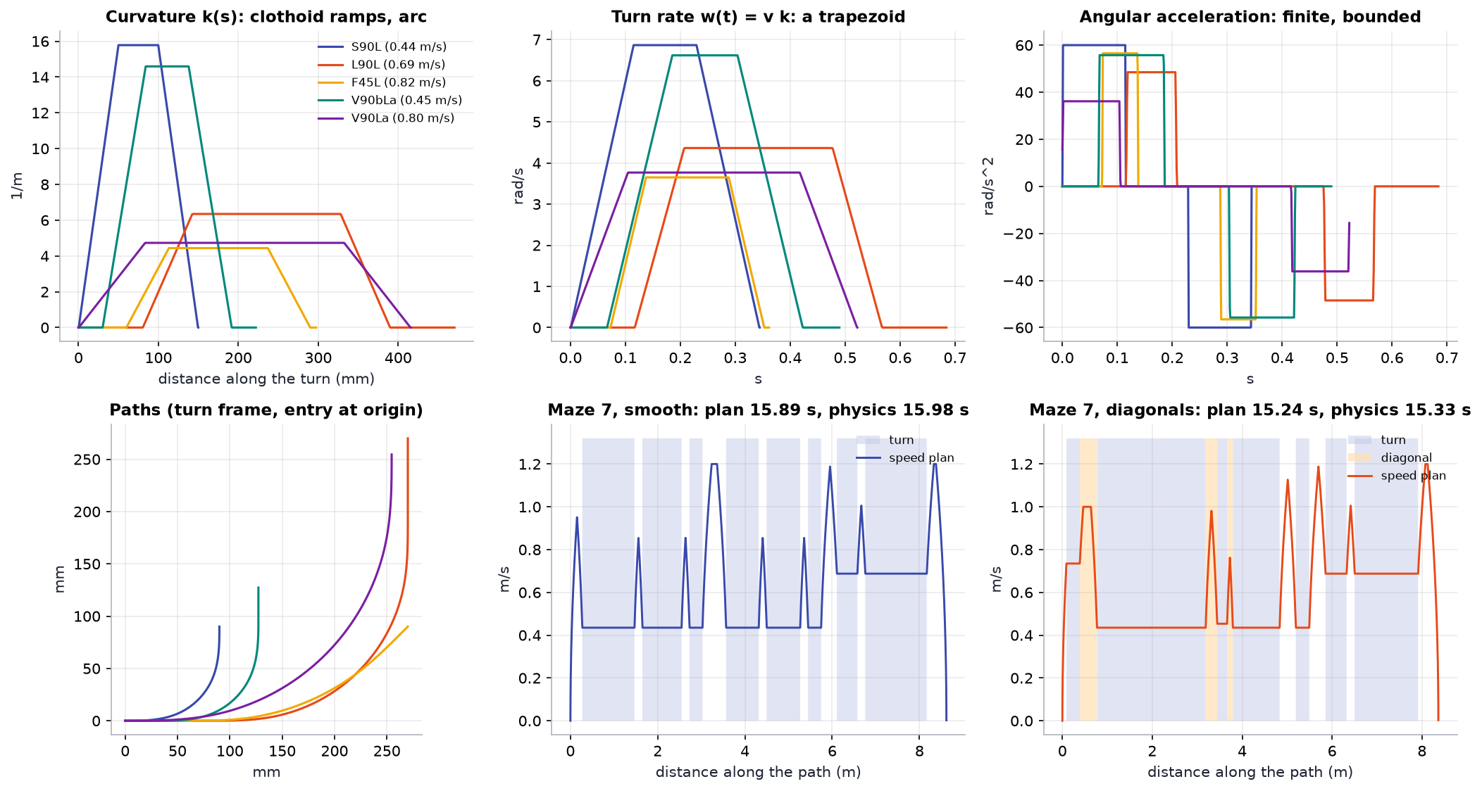
With ramp length \(L_c\) and arc length \(L_a\), the turn angle is \(\theta = \kappa_{max}(L_c + L_a)\); the ramp fraction \(f = L_c/(L_c + L_a)\) sets the shape. Curvature changes linearly with distance on the ramps, so the turn rate \(\omega = v\,\kappa(s)\) is a trapezoid in time and the angular acceleration on the ramps,
is finite. A plain arc would need an infinite one. The heading has a closed form (quadratic on the ramps, linear on the arc),
with \(s_1 = s - p\), which the firmware evaluates every tick, so every turn rotates by exactly its angle whatever the step size.
The shape is self-similar: for a given \(\theta\) and \(f\), the curve just scales with \(1/\kappa_{max}\). Its end point \((x_t, y_t)\) is computed once for \(\kappa_{max} = 1\) and scaled. Landing on the exit pose \((X, Y)\) then fixes the straights:
and a design is valid when \(p \ge 0\) and \(q \ge 0\).
Poses on edges
Positions are in half-cell units, so every edge midpoint has integer coordinates. An orthogonal pose crosses its edge square-on, a diagonal pose at 45 degrees. A turn is designed in a canonical frame: entry at the origin heading +x (orthogonal, 'O') or heading 45 degrees through a vertical edge ('A') or a horizontal edge ('B'). 'A' and 'B' are different problems: the grid is not symmetric about the 45 degree line through the entry, so a left turn from 'A' is the mirror image of a right turn from 'B', not of a left turn from 'A'. Orthogonal right turns are mirror images of the left ones.
The designer
For each turn class (orthogonal 90, 45 and 135 in; diagonal 45 and 135 out; diagonal-to-diagonal 90) and every exit edge within three cells, a grid search over \(\kappa_{max}\) and \(f \in [0.25, 1]\) keeps the design with the highest speed cap
subject to clearance: the 95 x 80 mm body is swept along the path (4 mm steps, then re-checked at 1 mm) against every post and against a wall on every edge the centre path does not cross. That is the worst maze the turn can ever meet, so if the edges a turn crosses are open, the turn fits. A design must keep 12 mm from everything.
From the designs, any one that is just another design plus straights (and not more than 3 % faster) is dropped, and the two fastest remain per class: 30 turns in all.
| Turn (left, flavour A) | Angle | \(R_{min}\) | Ramp \(f\) | Clearance | \(v_{cap}\) at 3 m/s² |
|---|---|---|---|---|---|
| S90: corner of the next cell | 90 | 63 mm | 0.50 | 21.9 mm | 0.44 m/s |
| L90: over 2 x 2 cells | 90 | 158 mm | 0.25 | 12.1 mm | 0.69 m/s |
| F45: orthogonal to diagonal | 45 | 225 mm | 0.30 | 12.0 mm | 0.82 m/s |
| F135 / F135b | 135 | 177 / 81 mm | 0.25 / 0.30 | 12.4 / 12.2 mm | 0.73 / 0.49 m/s |
| D45: diagonal to orthogonal | 45 | 225 mm | 0.30 | 12.0 mm | 0.82 m/s |
| D135 / D135b | 135 | 177 / 81 mm | 0.25 / 0.30 | 12.4 / 12.2 mm | 0.73 / 0.49 m/s |
| V90 / V90b: diagonal to diagonal | 90 | 211 / 69 mm | 0.25 / 0.50 | 12.3 / 12.0 mm | 0.80 / 0.45 m/s |
python -m sim.turns prints all 30 with their crossed edges; --plot draws them.
Why 12 mm and not 8. The first library used 8 mm. In Monte Carlo every diagonal-run failure happened in a turn designed at 8 mm, with the robot 8 mm or more off the path at that moment. At 12 mm the tight turns get about 10 % slower (V90b 0.49 to 0.45 m/s) and those failures went away for the designs; what remains is the heading error budget of section 14.
What limits the turns. Two different things, and the design studies separate them. The turns that pass close to a post (F45, V90b, D135b) are limited by clearance: the radius they can use, and through \(\sqrt{R}\) their speed, depends on the body width. S90 has 21.9 mm of clearance to spare and is limited by \(\alpha_{max}\) instead, and from \(a_{lat}\) = 4 m/s² so are 20 of the 30 turns. S90 is the turn the robot spends most time in, so a 64 mm body changes the mean run time by less than 1 % (width study), while \(\alpha_{max}\) = 80 rad/s² with \(a_{lat}\) = 4 m/s² saves 11 % (angular-acceleration study). The grip limit on angular acceleration is \(\alpha_{grip} = b\sqrt{(\mu g)^2 - a_{lat}^2}/2k^2\) for track \(b\) and radius of gyration \(k\): 83 rad/s² for this robot with \(\mu\) = 0.5.
12. Fast-run planner and speed plan
Code: sim/planner.py, MazeMap::planSmooth() and planSpeeds() in firmware/lib/mazecore.
Dijkstra over poses
States are (edge, heading): \((17\times16 + 16\times17)\) edges × 8 headings = 4352 for 16 × 16, plus a start (at rest in the start cell) and a goal. Moves: orthogonal straights over \(k\) edges, diagonal straights over \(k\) edges, every library turn whose crossed edges are known open, and "stop": from an edge into a goal cell, braking to rest at its centre.
Costs are integers in units of 0.1 ms from a simple speed model. Let \(v_n\) be the fastest allowed turn speed. A straight costs its time from \(v_n\) to \(v_n\) (trapezoid, capped at \(v_{max}\)); a turn of length \(L\) and speed \(v\) costs
where the second term is the time lost braking from \(v_n\) to \(v\) and accelerating back (exact when the neighbouring straights are long enough). Orthogonal-only runs ("smooth" mode) allow only the S90 and L90 turns.
The model is a ranking device, not a clock: over 60 random mazes it underestimates the exact time by 15 % on average (0.5 to 35 %): the formula is exact only when the straights between turns are long enough, and fast paths chain turns with short straights between them. It ranks close alternatives imperfectly, and the width study shows the cost: a library with faster turns lowered the search cost by 1.2 % while the exact time rose by 0.9 %. A search whose cost matches the speed plan is an open problem on the roadmap.
Speed plan
The chosen path becomes a segment list. Turns run at constant speed, straights accelerate or brake at \(a\). Boundary speeds \(b_i\) start at the segment limits; a forward pass and a backward pass apply
and a turn forces equal speeds at both ends. After both passes every constraint holds and no boundary speed can be raised. The total time of this profile is what the planner reports, and it is also exactly what the robot executes (section 13).
Python and C++ agree bit for bit
The C++ planner repeats the Python one operation for operation in double precision: same cost formulas, the same rounding to integer units, the same move order, and an indexed binary heap ordered by (cost, state id), which pops in the same order as Python's heapq of tuples. The native tests check, on the four test mazes with and without diagonals, that the Dijkstra cost is identical, the command sequence is identical, the planned time agrees to 2 ms and the plan runner ends where Python's does. The planner's working memory is about 70 kB of static RAM on the ESP32; the firmware prints the planning time with the plan (serial p).
Results
Benchmark study, 200 random mazes, "normal" preset: smooth turns take 0.56 of the v1 pivot estimate on average; diagonals take 0.94 of smooth on average and 0.71 in the best maze. The v1 estimate is optimistic for pivots: on maze 7 it says 30.2 s where the physics model takes 39.5 s, against 16.0 s (smooth) and 15.3 s (diagonals) in physics (python -m sim.run compare).
13. Path following and the wall observer
Code: PlanExecutor, Robot._track, Robot._wall_observer in sim/robot.py; mcore::PlanRunner, trackRate, wallObserver in firmware/lib/motioncore; wired up in firmware/src/motion.cpp.
Plan runner
One continuous distance coordinate runs through all segments, so nothing is lost when a segment ends mid-tick. Speed: \(v \leftarrow \min\left(v + a\,\Delta t,\ v_{seg},\ \sqrt{v_{end}^2 + 2a\,d_{left}}\right)\); the speed plan guarantees that braking for the next boundary is always enough. Heading reference: the closed-form curve heading. The runner also integrates the reference pose (midpoint rule; exact on straights, micrometres per turn: the test compares it with the ideal path).
Why path following
The first version steered on the straights exactly like v1 (raw side-wall offset) and ran turns open loop. The simulator showed the robot drifting 2 to 3 mm further from the plan at every turn: short straights between turns end with the wall-steering correction half done, the heading is about a degree off when the next turn starts, and the whole turn runs rotated. The fix is to follow the planned path everywhere, turns included, with the same law as section 6:
but with \(e\) and \(\psi\) the cross-track and heading errors of the pose estimate (encoders plus gyro) against the reference pose. With the walls feeding the pose estimate instead of the steering directly, the error no longer accumulates.
Wall observer
On orthogonal straights the planned path is the corridor centre line, so the side sensors measure the true cross-track error. Per metre travelled (\(s\)), with \(\psi\) the heading error and \(\beta\) the heading drift per metre caused by gyro bias:
Each fresh ToF sample feeds the innovation \(r = e_{wall} - \hat e\) into offset, heading and bias:
where \(D\) is the distance since the previous sample. The error dynamics are then \((\lambda + 1/L)^3\) in the distance domain: a triple pole at \(-1/L\) per metre, \(L = 1\) m. Innovations above 20 mm are rejected (wall ends, posts).
- Distance, not time. A time-domain version with the same structure learned a gyro bias of -0.0026 rad/s on the very first straight, where the true bias was zero: at low speed, time-based gains turn sensor noise into heading and bias. In the distance domain the gains vanish at standstill, which is right, because then the walls say nothing about heading.
- It learns the gyro bias. On the four test mazes with a true bias of +-0.002 rad/s, the estimate ends between 0.0016 and 0.0024 with the right sign every time (
test_wall_observer_learns_the_gyro_bias). - L = 1 m came from Monte Carlo: L = 0.5 m let ToF noise (3 mm per reading) into the heading; L = 2 m corrected too slowly; no observer at all (L very large) finished 12 % of smooth runs under the stress gyro errors.
Front wall. When the map says a wall closes the cell after a straight, the front sensors measure how far along the robot really is. The along-track error (from wheel radius tolerance, 0.3 % of 10 m is 30 mm) is fed into the distance loop with a gain of \(1 - e^{-D/0.08\,\text{m}}\) per sample, again per distance so it works at any sensor rate.
Physics additions in v2
- Friction circle. Each tyre gives whatever sideways force keeps the robot from sliding, up to what the friction limit leaves after the drive force; beyond that the body slides (body frame: \(\dot v_y = F_y/m - \omega v\), with \(|F_y| \le \sum_{wheels} \sqrt{(\mu N)^2 - F_x^2}\)). A smooth turn taken too fast slides out of its line (
test_too_fast_turn_slides_out). With \(a_{lat} = 3\) m/s² against \(\mu g = 4.9\) to 8.8 m/s² in the Monte Carlo, the presets do not slide; the speed–reliability study pushes \(a_{lat}\) until they do. - Gyro scale error (
gyro_scale) and the firmware's correction (gyro_k). - ToF beam cone (section 10).
14. Gyro calibration, and what diagonals need
A gyro scale error \(\varepsilon\) turns every turn of angle \(\theta\) into \(\theta(1 + \varepsilon)\). Smooth orthogonal runs get the error back from the walls on the next straight. Diagonals do not see walls, and the diagonal corridor between posts leaves 15 mm a side, so the heading error accumulated since the last walled straight decides whether a diagonal run survives.
The gyro study sweeps the residual scale error over 32 randomised robots per point. Smooth orthogonal runs finish 32 of 32 at every value. Diagonal runs hold at 28 to 30 of 32 up to \(\pm 0.15\,\%\) and fall to 20 of 32 at \(\pm 0.3\,\%\). Diagonals need the scale calibrated to about 0.15 %, which the calibration mode reaches with margin. The failures that remain below that are concentrated in one maze (seed 1), which fails even with a perfect scale: a property of its tight turn sequence, not of the estimator, and the motivation for risk-aware planning on the roadmap.
Calibration mode ("calibrate gyro scale"): start in a cell with a wall in front; the robot squares up, spins whole turns on the gyro and reads the angle left over on the front wall, \(f_l - f_r = 2 \times 20\ \text{mm} \times \tan\delta\). True over measured rotation is the scale error. It spins 1 turn, then 4, then 20, so the leftover angle stays small enough for the front sensors at every stage (one turn with a 3 % error leaves 11 degrees; going straight from 1 to 20 turns left up to 29 degrees, which the sensors misread). python -m sim.calibrate runs the same routine on the simulated robot: from a 3 % start the residual is within +-0.063 % over 12 runs, median about 0.02 %. Run it three times; keep it if the results agree within 0.03 %.
Gyro bias is measured at power-up (500 samples), measured again at the start of every run while the robot stands still (400 ms), and learned during the run by the wall observer (section 13).