Design studies

Every number on this site comes from one of the studies below. Each is a function in sim/studies.py that writes a figure and a data file; the charts on this page are drawn from those files and are interactive (hover, zoom, toggle series).

python -m sim.studies all      # about 45 minutes on 12 cores; or one study by name
python -m sim.studies site     # rebuild the interactive charts from the data

Method: robots, errors and confidence intervals

Robots. Every physics run randomises the robot: mass −10 % to +15 %, tyre friction \(\mu \in [0.5, 0.9]\), battery 7.0 to 8.2 V, each motor constant \(\pm 10\,\%\), wheel radii and track width \(\pm 0.3\,\%\) (after the calibration modes). The controller always uses the gains designed for the nominal robot, as the real firmware does.

Error models.

	gyro bias (1 σ)	gyro scale residual	wall sensors
realistic	0.0005 rad/s (re-zeroed at the start; in-run thermal drift)	uniform ±0.06 % (after the calibration mode)	VL53L0X: 30 Hz, 3 mm noise, 25° cone
stress	0.002 rad/s	uniform ±0.3 %	same

Mazes. Four generated 16 × 16 mazes (seeds 7, 42, 1, 2025) with 8 robots each, so 32 runs per configuration. A run finishes if the robot never touches a wall or post and stops in the goal.

Intervals. Finish rates are shown with 95 % Wilson score intervals,

\[ \frac{\hat p + \frac{z^2}{2n} \pm z\sqrt{\frac{\hat p(1-\hat p)}{n} + \frac{z^2}{4n^2}}}{1 + \frac{z^2}{n}}, \qquad z = 1.96 \]

which stay honest at small \(n\) and near 0 or 100 %: 32 of 32 means "at least 89 %", not "100 %".

Control loops

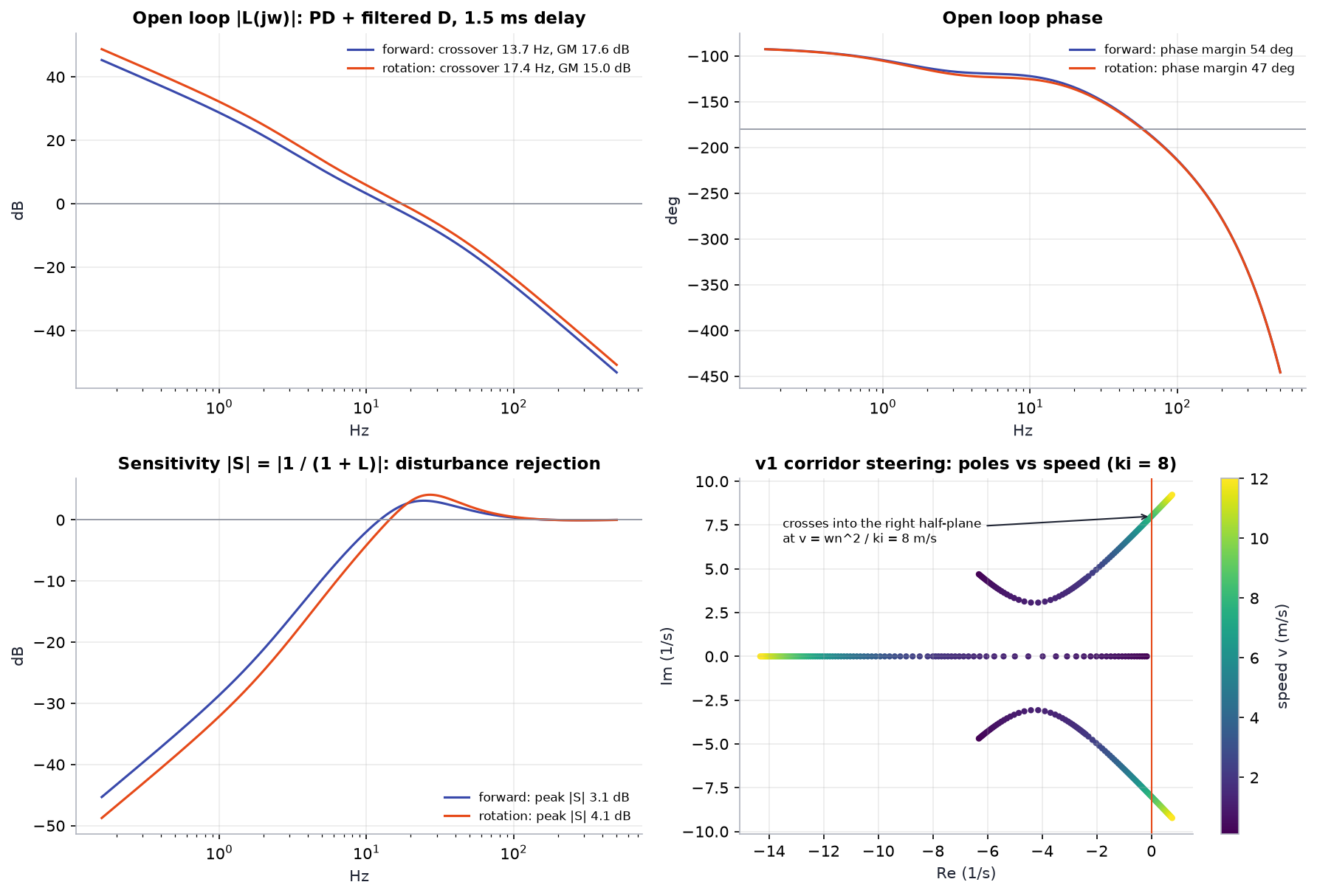
Loop	Crossover	Phase margin	Gain margin	Peak sensitivity
forward (position)	13.7 Hz	54°	17.6 dB	3.1 dB
rotation (heading)	17.4 Hz	47°	15.0 dB	4.1 dB

The open loop includes the plant \(K / (s(s + 1/\tau))\), the PD controller with its 4 ms derivative filter, and a 1.5 ms delay (half a sample of zero-order hold plus one sample of computation). Both loops have comfortable margins; the sensitivity peaks below 4.1 dB mean a disturbance is amplified by at most 1.6× anywhere in frequency. The root locus shows the v1 corridor-steering loop with its heading-bias integrator: a complex pair moves right with speed and crosses into the right half-plane at exactly \(v = \omega_n^2 / k_i = 8\) m/s, the Routh–Hurwitz bound derived in the notebook.

Turn and speed profiles

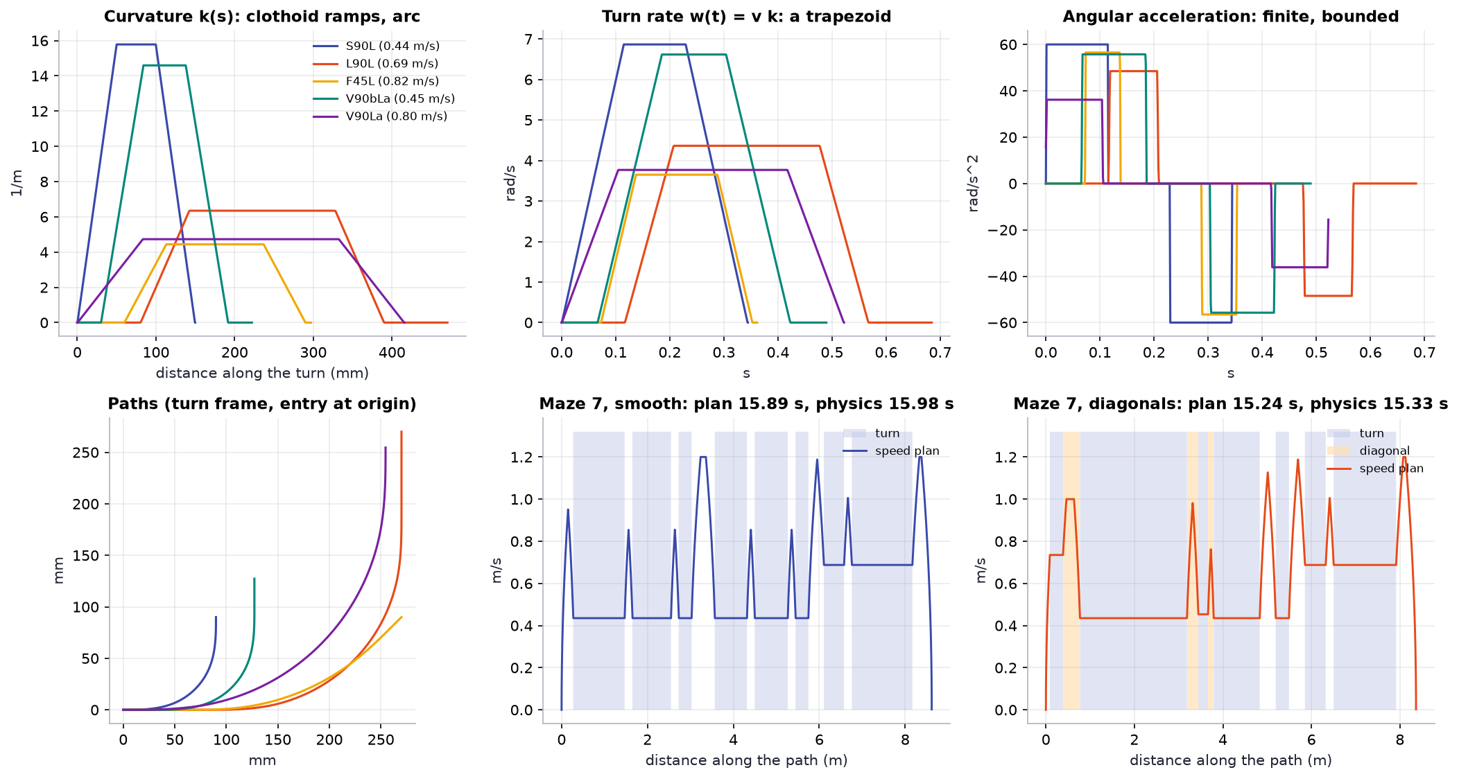
The top row is what makes the turns drivable: curvature ramps linearly (clothoids), so the turn rate is a trapezoid and the angular acceleration is bounded instead of infinite. The speed plan of maze 7 shows the real bottleneck: most of the run is spent at turn speed (0.44 m/s through S90 turns, 0.69 m/s through L90 turns), with short bursts to 1.2 m/s on straights. Faster turns, not a higher top speed, are what shortens the run. The last three studies find out what actually limits turn speed: grip, chassis width or angular acceleration.

The planned and physics times agree to within 0.1 s (15.89 vs 15.98 s smooth, 15.24 vs 15.33 s with diagonals): the speed plan is what the robot actually executes, plus the final settling.

Planned run times

19.5 smedian planned time, stop-and-pivot (v1 cost model, optimistic)

10.7 smedian, smooth turns

10.0 smedian, with diagonals

−29 %best diagonal saving over smooth turns (mean −6 %)

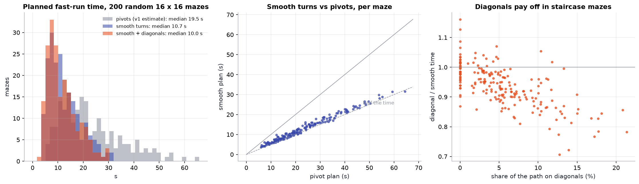
Smooth turns take 0.56 of the pivot plan's time on average over 200 mazes, and the v1 cost model is optimistic for pivots (on maze 7 it predicts 30.2 s where the physics model takes 39.5 s). Diagonals pay off in proportion to how much of the path is a staircase; in mazes without staircases they change nothing.

Reliability

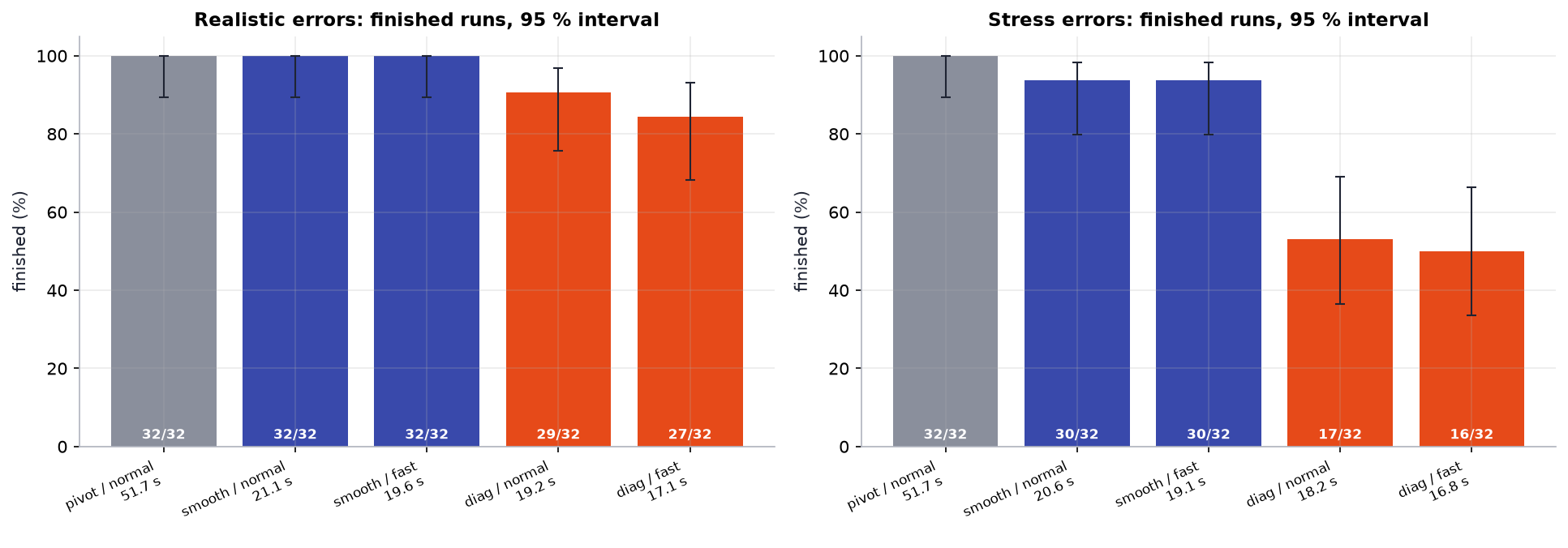
Fast run	Preset	Realistic: finished	Stress: finished	Mean time	Path error RMS (realistic)
stop-and-pivot (v1)	1.2 m/s	32 / 32 [89, 100] %	32 / 32 [89, 100] %	51.7 s
smooth turns	normal	32 / 32 [89, 100] %	30 / 32 [80, 98] %	21.1 s	1.5 mm
smooth turns	fast	32 / 32 [89, 100] %	30 / 32 [80, 98] %	19.6 s	1.5 mm
with diagonals	normal	29 / 32 [76, 97] %	17 / 32 [36, 69] %	19.2 s	2.7 mm
with diagonals	fast	27 / 32 [68, 93] %	16 / 32 [34, 66] %	17.1 s	2.8 mm

Smooth turns are the default fast run

2.4× faster than stop-and-pivot, every realistic run finished, and the real robot stays within 1.5 mm RMS of the planned path. Under the stress errors the two failures are both in maze 1.

Diagonals are opt-in

They are faster but leave the robot with no wall beside it for long stretches, so heading errors accumulate. Under stress errors they fail half the time.

Gyro calibration and diagonals

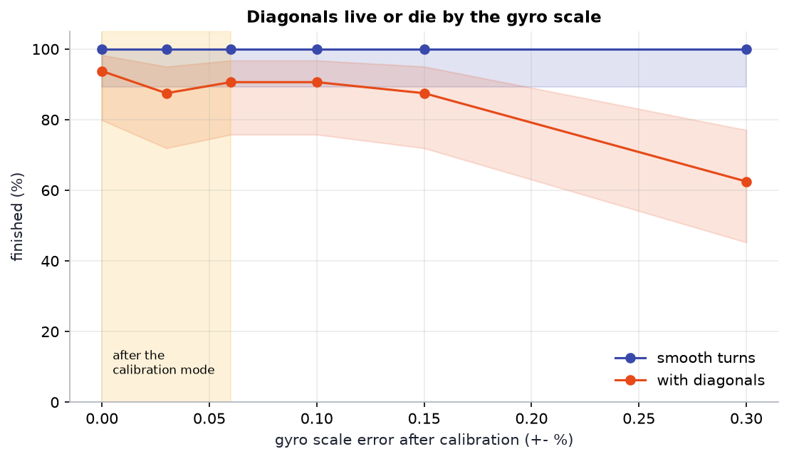
Smooth runs finish 32 of 32 at every scale error tested: the walls on the next straight remove any heading error. Diagonal runs hold at 28 to 30 of 32 up to \(\pm 0.15\,\%\) and fall to 20 of 32 at \(\pm 0.3\,\%\), so the calibration mode's 0.06 % is enough. The failures below 0.15 % are concentrated in one maze (seed 1 finishes 4 to 6 of 8 even with a perfect gyro, the other three mazes 8 of 8): a tight sequence of turns in that maze, not the estimator. That points at the next research step, planning that accounts for risk as well as time.

Wall sensors: ToF against pulsed IR

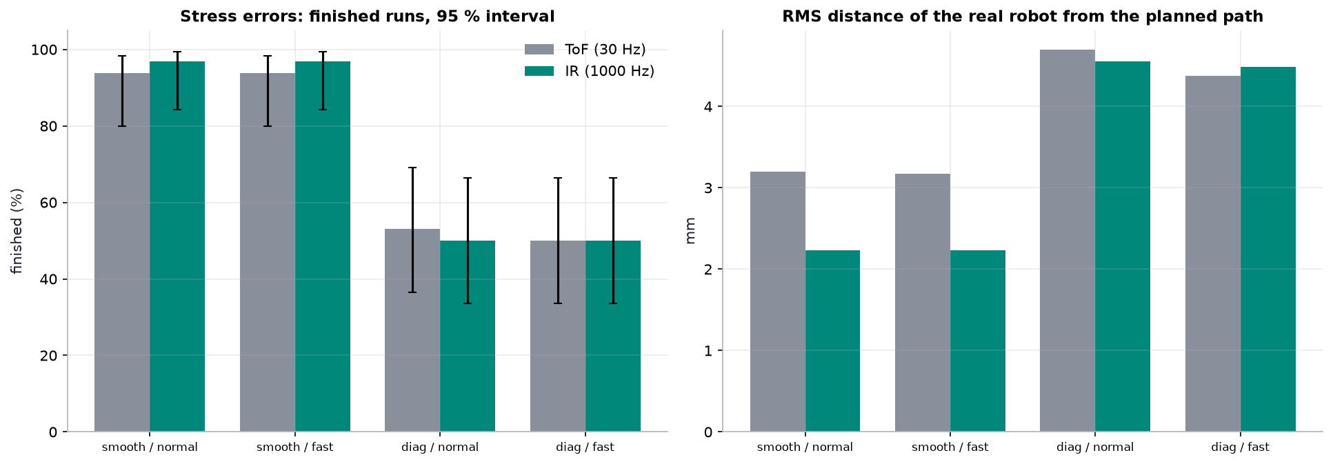
The same robots, stress errors, once with the VL53L0X model (30 Hz, 3 mm noise, 25° cone) and once with the Mk II pulsed-IR model (1 kHz, 1 mm noise, narrow spot, same mounting). Because the wall observer's gains are per metre travelled, not per sample, the same code runs at either rate unchanged.

Fast run	Sensor	Finished	Path error RMS	Median worst-case error
smooth, normal	ToF	30 / 32 [80, 98] %	3.2 mm	6.6 mm
smooth, normal	IR	31 / 32 [84, 99] %	2.2 mm	4.6 mm
diagonals, normal	ToF	17 / 32 [36, 69] %	4.7 mm	13.8 mm
diagonals, normal	IR	16 / 32 [34, 66] %	4.6 mm	13.9 mm

On smooth runs the faster, quieter sensor cuts the path error by 30 %, both on average and in the worst case. On diagonals it changes nothing, and that is the useful finding: on a diagonal there is no wall beside the robot, so the side sensors only see posts flashing past, and the current observer ignores them. With a 1 kHz sensor those post edges can be timed to a millimetre and become position fixes; with a 30 Hz sensor they cannot. Faster sensors are necessary for good diagonals, but the estimator has to change too: that is milestone M5 on the roadmap.

Speed against reliability

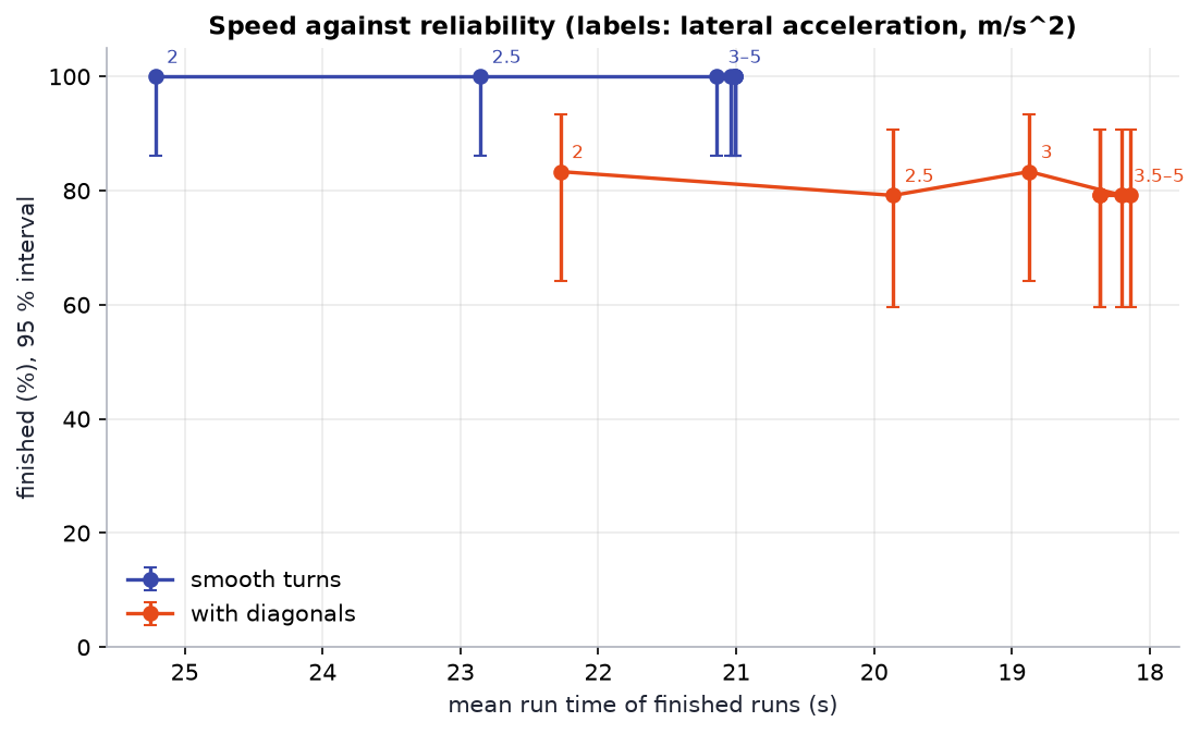
The lateral-acceleration limit \(a_{lat}\) swept from 2 to 5 m/s², everything else at the normal preset (1.2 m/s straights, 3 m/s² acceleration, 60 rad/s² angular acceleration); 24 randomised robots per point, realistic errors.

\(a_{lat}\) (m/s²)	Smooth: finished	Smooth: mean time	Diagonals: finished	Diagonals: mean time
2.0	24 / 24	25.2 s	20 / 24	22.3 s
2.5	24 / 24	22.9 s	19 / 24	19.9 s
3.0 (normal)	24 / 24	21.1 s	20 / 24	18.9 s
3.5	24 / 24	21.0 s	19 / 24	18.2 s
4.0 to 5.0	24 / 24	21.0 s	19 / 24	18.1 to 18.4 s

The time stops improving at about 3.5 m/s², and it is not grip that stops it. A turn's speed has two caps: grip in the arc, and how fast the turn rate may ramp up along the entry clothoid of length \(L_c\):

\[ v \le \sqrt{\frac{a_{lat}}{\kappa_{max}}}, \qquad \dot\omega = v^2 \frac{d\kappa}{ds} = v^2 \frac{\kappa_{max}}{L_c} \le \alpha_{max} \;\Rightarrow\; v \le \sqrt{\frac{\alpha_{max} L_c}{\kappa_{max}}} \]

Turn speed cap (m/s) at \(a_{lat}\)	S90	L90	F45	V90b	D135b
2 m/s²	0.36	0.56	0.67	0.37	0.40
3 m/s²	0.44 \(\alpha\)	0.69	0.82	0.45	0.49
4 m/s² and above	0.44 \(\alpha\)	0.76 \(\alpha\)	0.85 \(\alpha\)	0.47 \(\alpha\)	0.53 \(\alpha\)

(\(\alpha\): capped by angular acceleration.) S90, the turn the robot spends most of its time in, is already on the angular-acceleration cap at the normal preset; from 4 m/s² 20 of the 30 turns are, including every tight one (only the wide F135, D135 and V90 variants are still limited by grip). Smooth runs use only S90 and L90, so past 4 m/s² raising \(a_{lat}\) changes nothing for them, which is also why there is no reliability cost: the robots never actually reach the higher lateral limit. The lever that is left is \(\alpha_{max}\), swept below.

Diagonal reliability does not depend on speed. It holds at 19 to 20 of 24 at every setting, and the failures sit in the same two mazes every time (seed 1: 2 to 3 of 6, seed 2025: 5 of 6). Driving diagonals more slowly does not make them safer; better position estimates do, as the gyro and sensor studies show.

Chassis width

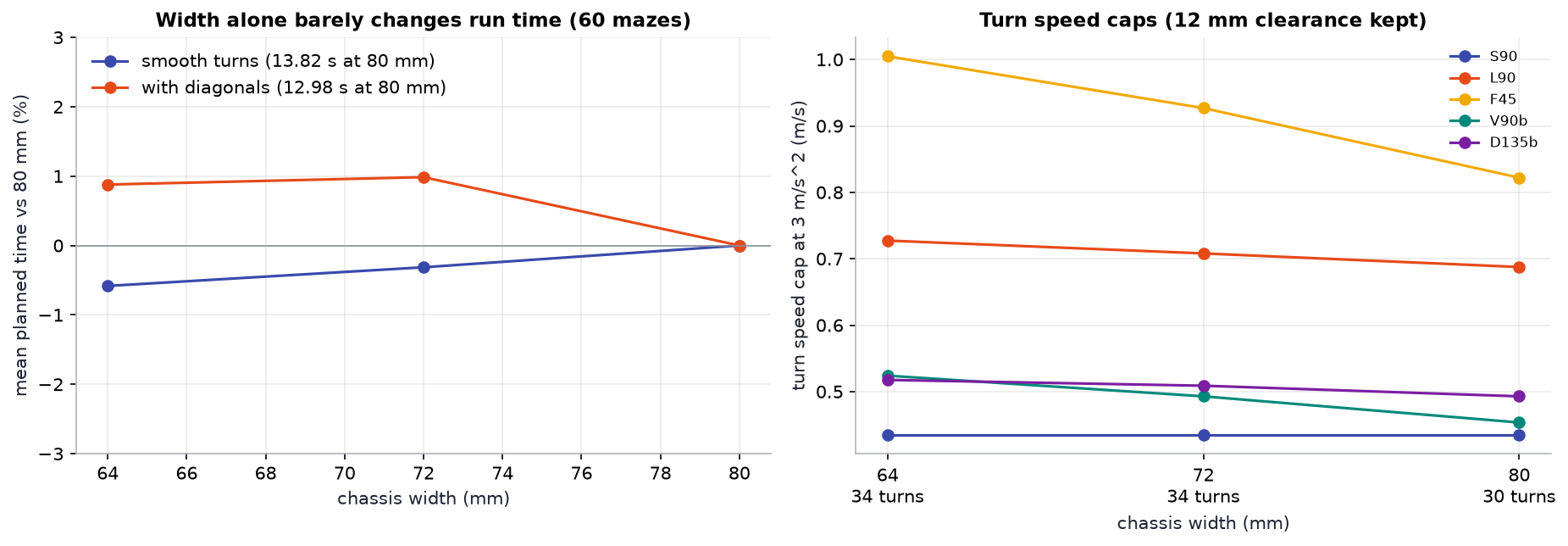
The turn designer is rerun for 64, 72 and 80 mm bodies (95 mm long, the same 12 mm worst-case clearance), and each library is planned on 60 random mazes at the normal preset. Turn speed caps in m/s at 3 m/s²:

Width	Turns	S90	L90	F45	V90b	D135b	Smooth: mean planned	Diagonals: mean planned
80 mm (Mk I)	30	0.44	0.69	0.82	0.45	0.49	13.82 s	12.98 s
72 mm	34	0.44	0.71	0.93	0.49	0.51	13.78 s	13.11 s
64 mm	34	0.44	0.73	1.00	0.52	0.52	13.74 s	13.10 s

Width alone is not worth chasing. A narrower body raises the caps of the turns that pass close to a post (F45 +22 %, V90b +16 %) and makes four more turns feasible (F45b and D45b), yet the mean run time moves by less than 1 %. S90, where the robot spends most of its turning time, has clearance to spare and is capped by angular acceleration, so it does not change at all.

The diagonal runs even get 0.9 % slower, and the reason is worth knowing. The path search minimises an approximate cost (each turn priced against the fastest turn speed \(v_n\), notebook §12); the exact time comes from the speed plan afterwards. With the 64 mm library the search's cost drops by 1.2 %, but in 27 of the 60 mazes the route it prefers is slower once the speed plan is exact. The approximate cost underestimates the exact time by 15 % on average (0.5 to 35 %), so it ranks close alternatives badly. A search cost that matches the speed plan is now on the research list.

This changed the Mk II brief. The PCB chassis is still narrower, because the same turns then pass up to 8 mm further from the posts (the diagonal failures in the notebook began 8 mm off the path), but the speed has to come from somewhere else.

Angular acceleration

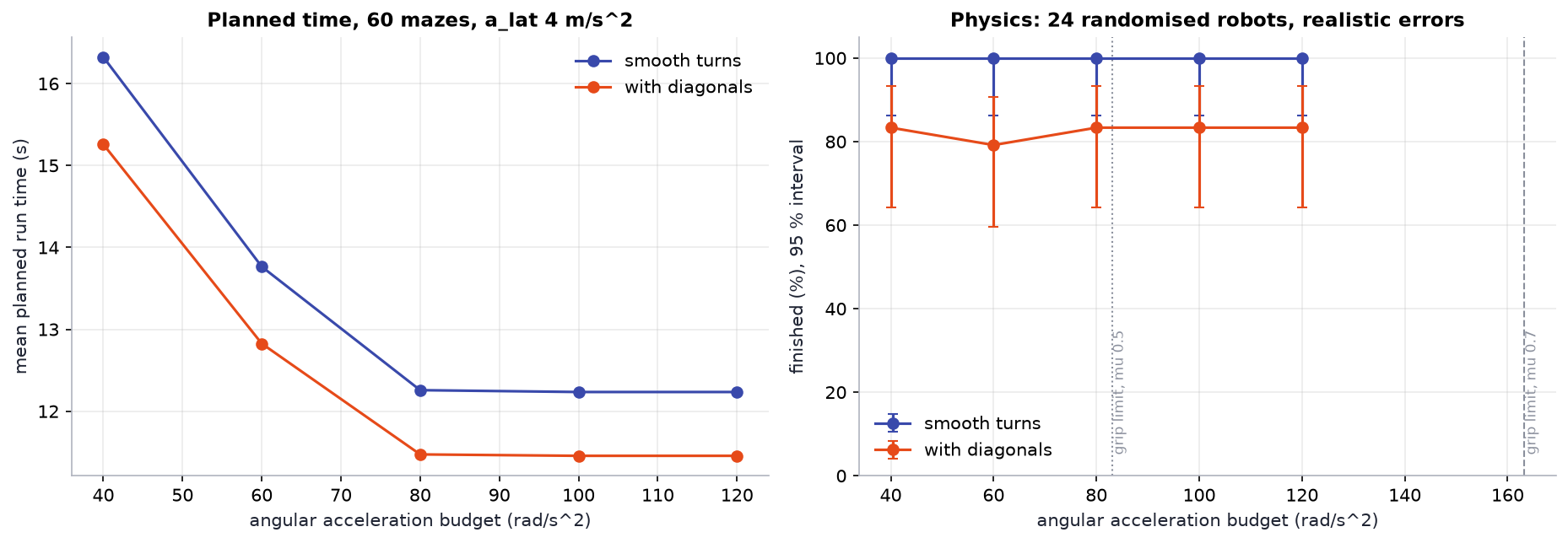
The angular-acceleration budget \(\alpha_{max}\) swept from 40 to 120 rad/s² at \(a_{lat}\) = 4 m/s² (so that grip is not the first cap), planned on 60 random mazes and driven in physics by 24 randomised robots per point, realistic errors.

\(\alpha_{max}\) (rad/s²)	Smooth: planned	Smooth: physics	Diagonals: planned	Diagonals: physics
40	16.32 s	24 / 24, 25.0 s	15.26 s	20 / 24, 22.0 s
60 (normal)	13.76 s	24 / 24, 21.0 s	12.83 s	19 / 24, 18.1 s
80	12.26 s	24 / 24, 18.7 s	11.47 s	20 / 24, 16.7 s
100	12.23 s	24 / 24, 18.6 s	11.46 s	20 / 24, 16.7 s
120	12.23 s	24 / 24, 18.6 s	11.46 s	20 / 24, 16.7 s

This is the lever. From 60 to 80 rad/s² the smooth run gets 11 % faster, planned and in physics, with every robot still finishing; past 80 nothing changes, because the turns are back on the grip cap \(\sqrt{a_{lat}/\kappa_{max}}\). The two caps have to rise together.

How much can the hardware give? Each wheel can push along the floor with what its friction circle has left after carrying its share of the lateral force; pushing in opposite directions across the track \(b\) gives

\[ \alpha_{grip} = \frac{F_{long}\, b}{J} = \frac{b}{2k^2}\sqrt{(\mu g)^2 - a_{lat}^2}, \qquad J = m k^2 \]

The mass cancels: only the track \(b\) and the radius of gyration \(k\) matter. For Mk I (\(b\) = 72 mm, \(k\) = 35 mm) at 4 m/s² that is 83 rad/s² with the worst tyres in the Monte Carlo (\(\mu\) = 0.5) and 163 rad/s² at \(\mu\) = 0.7 (the grey lines). The motors are not the limit: at turn speeds they can push 1.2 to 1.5 N per wheel, against 0.36 N of grip at \(\mu\) = 0.7.

In simulation, Mk I has headroom

\(a_{lat}\) = 4 m/s² with \(\alpha_{max}\) = 80 rad/s² finishes every smooth run and saves 11 %, and stays inside the grip limit of even the worst tyres. Whether the real tyres have that grip is exactly what milestone M1 measures before any preset changes.

For Mk II this sets the layout rule: with the battery over the axle and the board as the chassis, \(k\) shrinks, and \(\alpha_{grip}\) grows with \(1/k^2\). A narrower track works against it, so the PCB keeps the wheels as far apart as the body allows.